Processing the data cube
The data cube in Fujita2023$data contains unprocessed counts. The
function processDataCube() performs the processing of these
counts with the following steps:
- It performs feature selection based on the sparsityThreshold setting. Sparsity is here defined as the fraction of samples where a microbial abundance (ASV/OTU or otherwise) is zero.
- It performs a centered log-ratio transformation of each sample using with a pseudo-count of one (on all features, prior to selection based on sparsity).
- It centers and scales the three-way array. This is a complex topic that is elaborated upon in our accompanying paper. By centering across the subject mode, we make the subjects comparable to each other within each time point. Scaling within the feature mode avoids the PARAFAC model focusing on features with abnormally high variation.
The outcome of processing is a new version of the dataset. Please
refer to the documentation of processDataCube() for more
information.
processedFujita = processDataCube(Fujita2023, sparsityThreshold=0.99, CLR=TRUE, centerMode=1, scaleMode=2)Determining the correct number of components
A critical aspect of PARAFAC modelling is to determine the correct
number of components. We have developed the functions
assessModelQuality() and
assessModelStability() for this purpose. First, we will
assess the model quality and specify the minimum and maximum number of
components to investigate and the number of randomly initialized models
to try for each number of components.
Note: this vignette reflects a minimum working example for analyzing
this dataset due to computational limitations in automatic vignette
rendering. Hence, we only look at 1-3 components with 5 random
initializations each. These settings are not ideal for real datasets.
Please refer to the documentation of assessModelQuality()
for more information.
# Setup
minNumComponents = 1
maxNumComponents = 3
numRepetitions = 5 # number of randomly initialized models
numFolds = 8 # number of jack-knifed models
ctol = 1e-6
maxit = 200
numCores= 1

# Plot settings
colourCols = c("", "Genus", "")
legendTitles = c("", "Genus", "")
xLabels = c("Replicate", "Feature index", "Time point")
legendColNums = c(0,5,0)
arrangeModes = c(FALSE, TRUE, FALSE)
continuousModes = c(FALSE,FALSE,TRUE)

# Assess the metrics to determine the correct number of components
qualityAssessment = assessModelQuality(processedFujita$data, minNumComponents, maxNumComponents, numRepetitions, ctol=ctol, maxit=maxit, numCores=numCores)
We will now inspect the output plots of interest for
Fujita2023.
qualityAssessment$plots$overview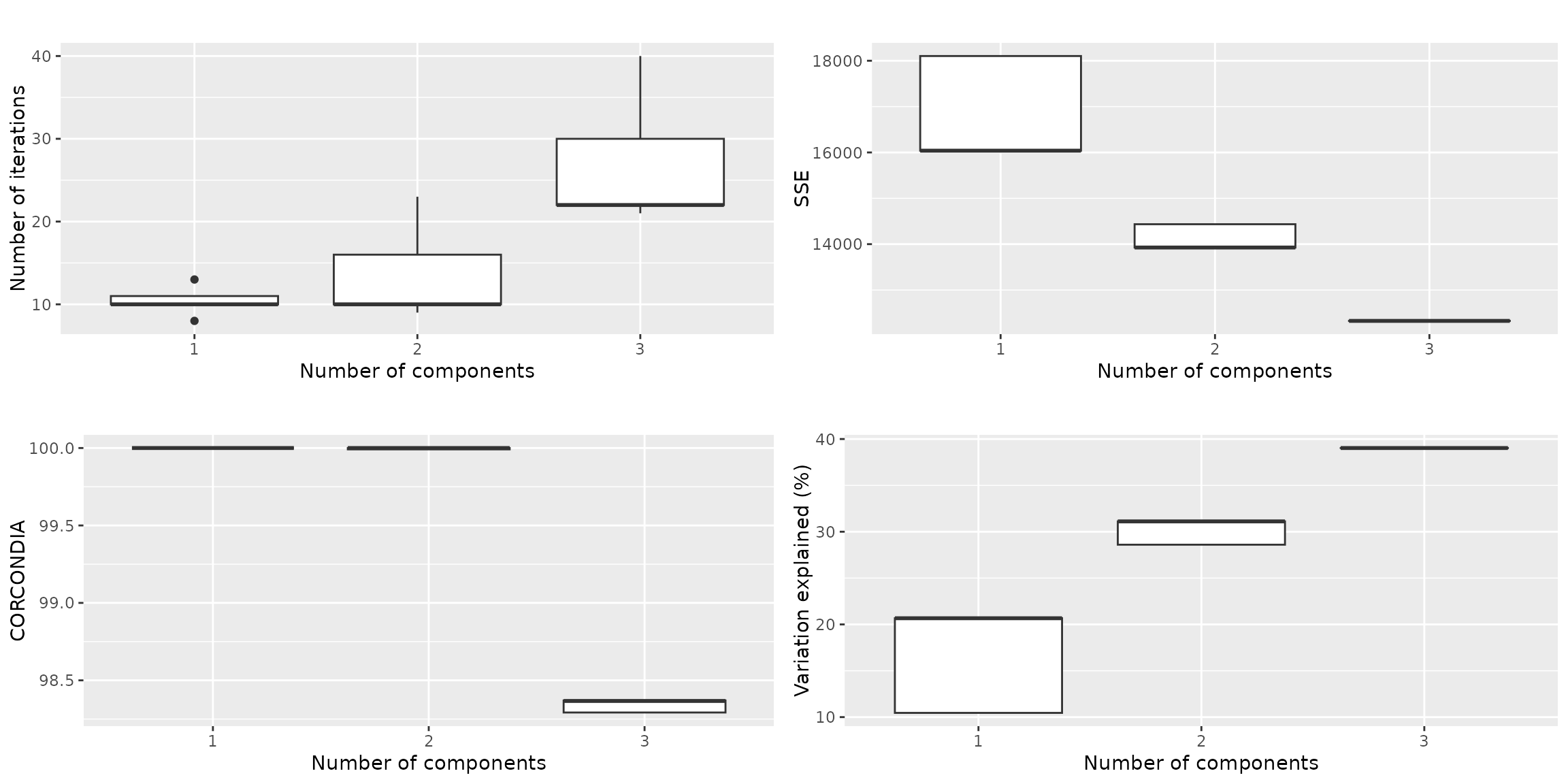 The overview plots show that we can reach ~40% explained variation if we
take 3 components. The CORCONDIA for those models are ~98, which is well
above the minimum requirement of 60. Based on this overview, either 2 or
3 components seems fine.
The overview plots show that we can reach ~40% explained variation if we
take 3 components. The CORCONDIA for those models are ~98, which is well
above the minimum requirement of 60. Based on this overview, either 2 or
3 components seems fine.
Jack-knifed models
Next, we investigate the stability of the models when jack-knifing
out samples using assessModelStability(). This will give us
more information to choose between 2 or 3 components.
stabilityAssessment = assessModelStability(processedFujita, minNumComponents=1, maxNumComponents=3, numFolds=numFolds, considerGroups=FALSE,
                                           groupVariable="", colourCols, legendTitles, xLabels, legendColNums, arrangeModes,
                                           ctol=ctol, maxit=maxit, numCores=numCores)
stabilityAssessment$modelPlots[[1]]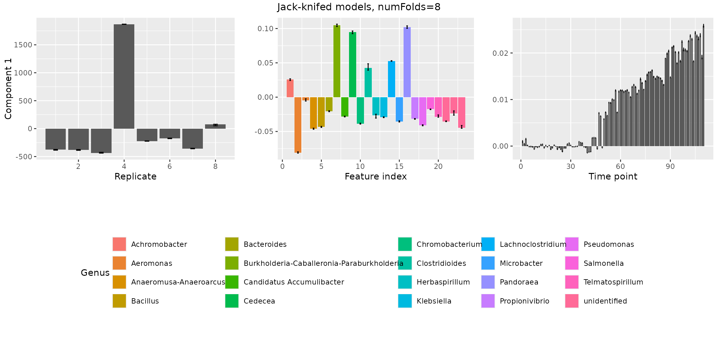
stabilityAssessment$modelPlots[[2]]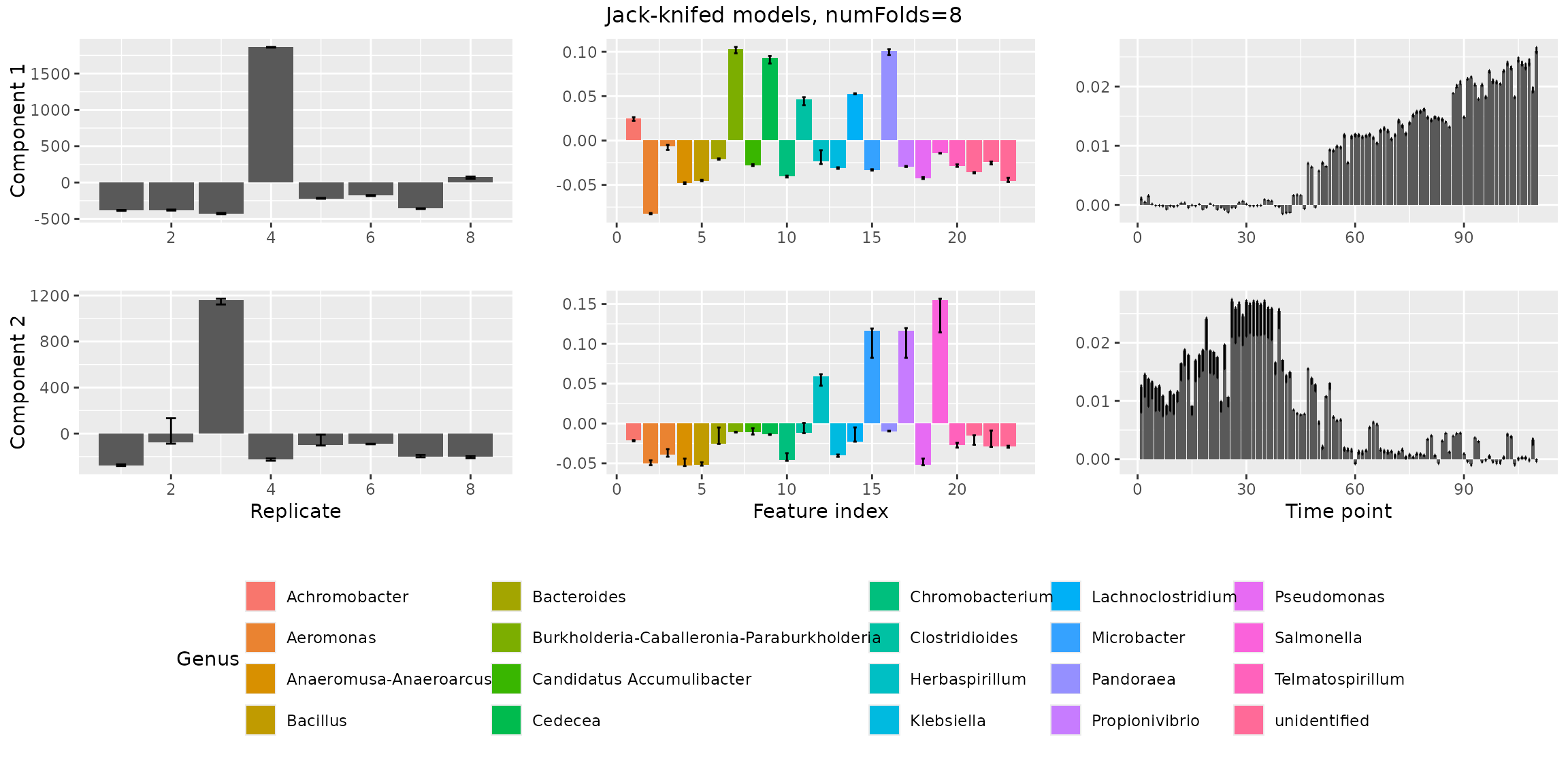
stabilityAssessment$modelPlots[[3]]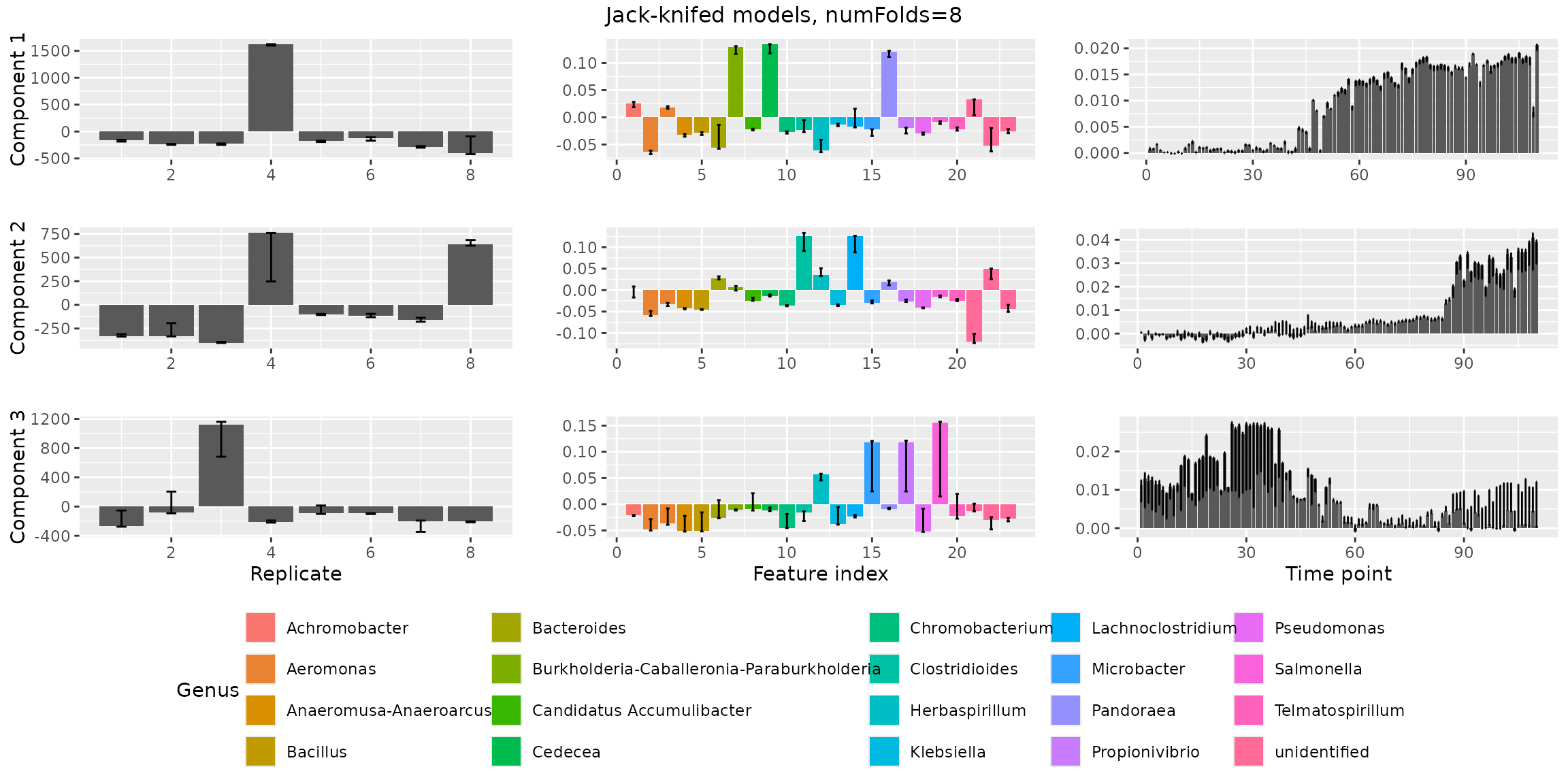 The three-component model is stable and can be safely chosen as the
final model.
The three-component model is stable and can be safely chosen as the
final model.
Model selection
We have decided that a three-component model is the most appropriate
for the Fujita2023 dataset. We can now select one of the
random initializations from the assessModelQuality() output
as our final model. We’re going to select the random initialization that
corresponded the maximum amount of variation explained for three
components.
numComponents = 3
modelChoice = which(qualityAssessment$metrics$varExp[,numComponents] == max(qualityAssessment$metrics$varExp[,numComponents]))
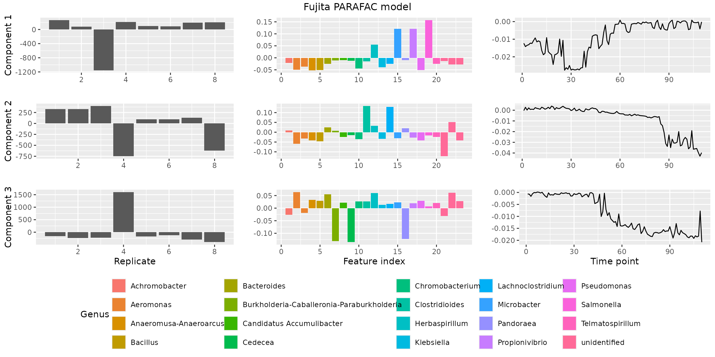
finalModel = qualityAssessment$models[[numComponents]][[modelChoice]]Finally, we visualize the model using
plotPARAFACmodel().
plotPARAFACmodel(finalModel$Fac, processedFujita, 3, colourCols, legendTitles, xLabels, legendColNums, arrangeModes,
  continuousModes = c(FALSE,FALSE,TRUE),
  overallTitle = "Fujita PARAFAC model")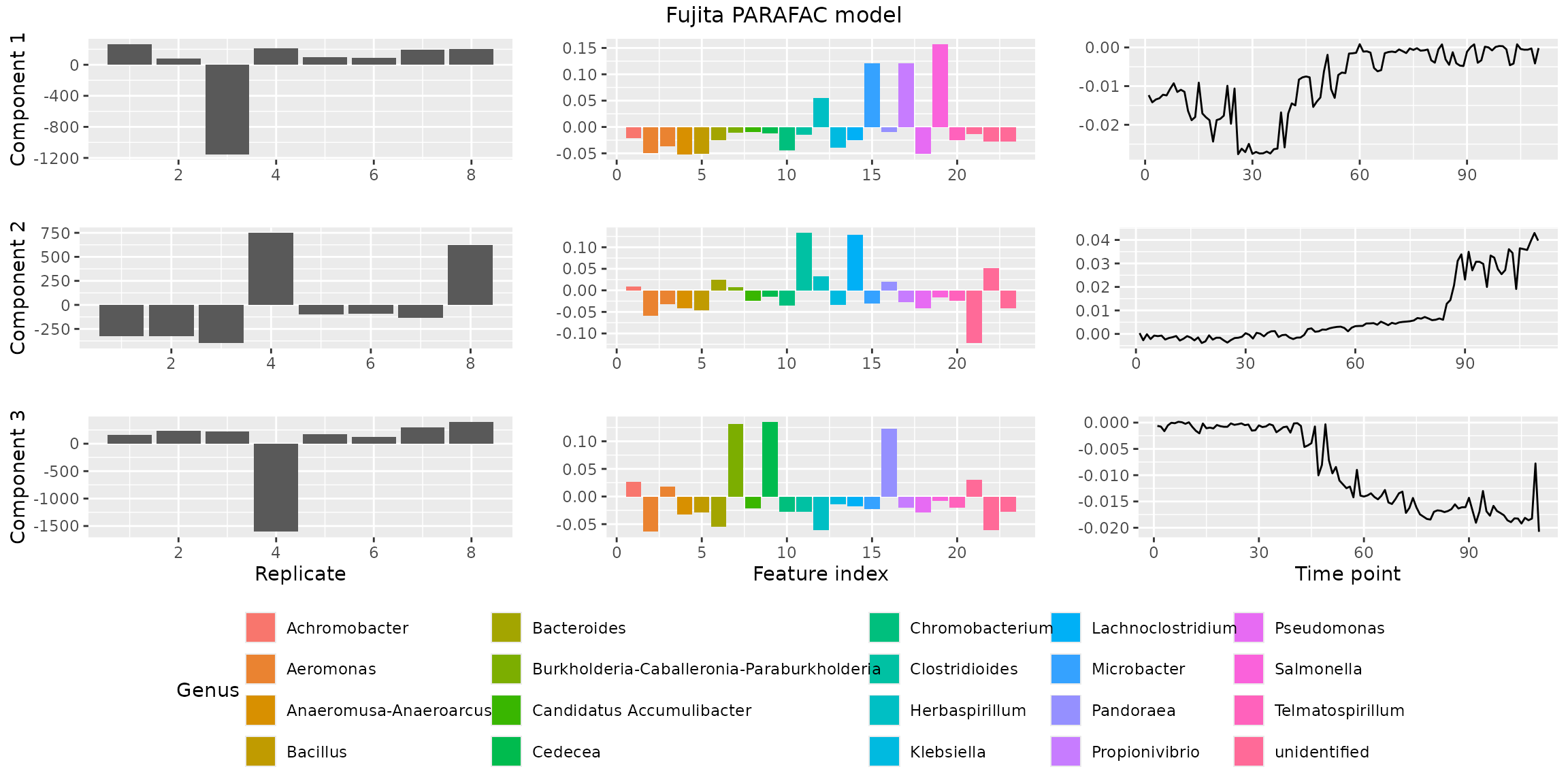
You will observe that the loadings for some modes in some components are negative. This is due to sign flipping: two modes having negative loadings cancel out but describe the same subspace as two positive loadings. We can manually sign flip these loadings to obtain a more interpretable plot.
finalModel$Fac[[1]][,2] = -1 * finalModel$Fac[[1]][,2] # mode 1 component 2
finalModel$Fac[[1]][,3] = -1 * finalModel$Fac[[1]][,3] # mode 1 component 3
finalModel$Fac[[2]][,3] = -1 * finalModel$Fac[[2]][,3] # mode 2 component 3
finalModel$Fac[[3]][,2] = -1 * finalModel$Fac[[3]][,2] # mode 3 component 2

plotPARAFACmodel(finalModel$Fac, processedFujita, 3, colourCols, legendTitles, xLabels, legendColNums, arrangeModes,
  continuousModes = c(FALSE,FALSE,TRUE),
  overallTitle = "Fujita PARAFAC model")